With the role of asset managers becoming increasingly important to the global financial services industry, it is important to look at the current market trends and how particular investment options impact asset manager’s returns.

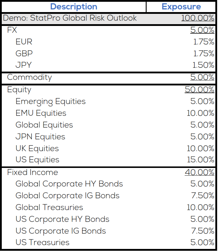
A sample portfolio is a useful tool to be able to see the impact such investment options have on a return where one can mirror the average asset manager allocation.

Below is a portfolio created to be globally diversified with assets across global FX, Commodity, Equity, and Fixed Income markets.

In this global risk outlook blog series, the sample portfolio will be rebalanced quarterly to maintain reporting integrity and will follow: 50% in global equities including emerging, and developed markets with bias towards US, UK and Europe, 40% in global fixed income spanning corporate, sovereign, high yield and investment grade, 5% in FX trading across EUR, GBP and JPY, and 5% in global commodities.

What happens when volatility returns?

The current bull market is approaching its ninth year; even if the first half of the upswing is removed, early 2009 through early 2013, the bull is still older than our last bull market from 2003 to 2007. With this bull market has come historic lows in the S&P Volatility Index (VIX) and a move from active managers to low-fee passive funds. Without volatility the value proposition of active managers is outweighed by the steady return of index funds at a lower cost. So, the question on everyone’s mind is this: when will market volatility return, and when will the aging bull market finally die?

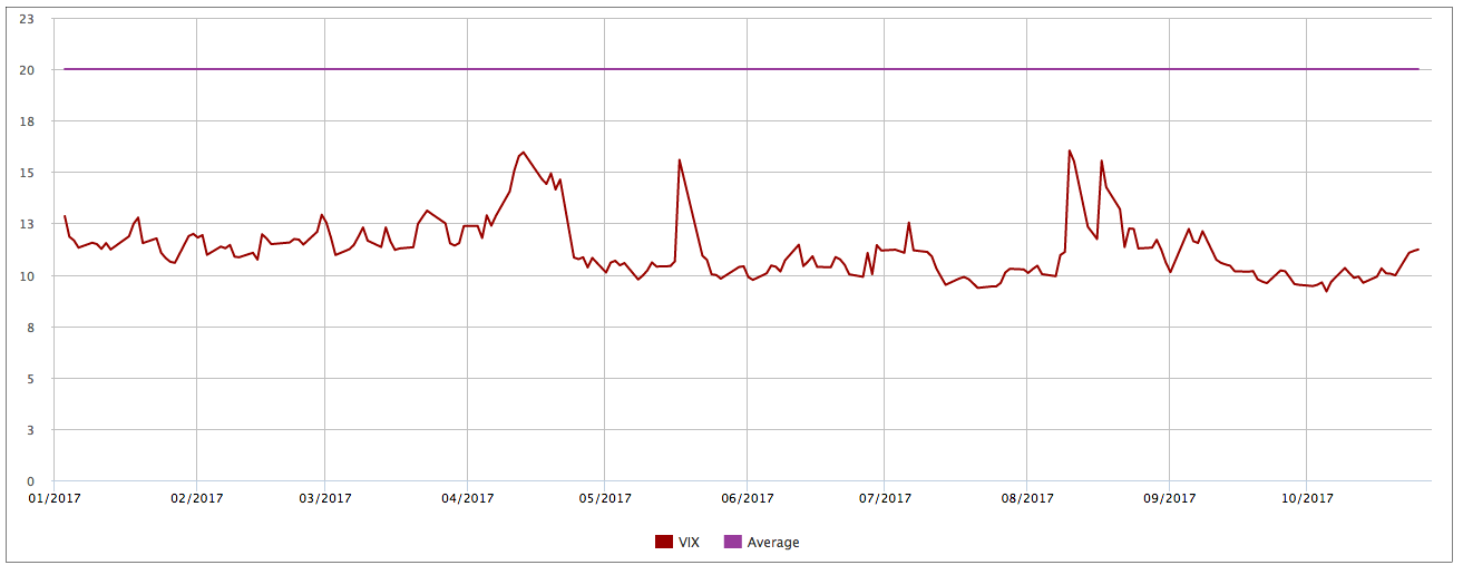
On October 5^th the S&P 500 reached a historic high of $2,552, while the VIX reached a record low of 9.19.  The year to date average* is not much higher, sitting at 10.8.  For reference, since the VIX was created in 1990, the average level is near 20.

_{Fig. 1: VIX price vs. Average since 1990}

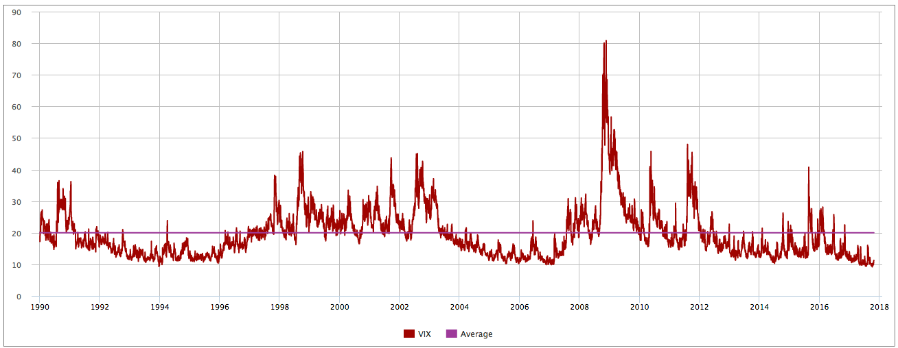
_{Fig. 2: YTD VIX price vs. historical average}

As you can see from Fig. 1, the VIX level tends to follow a smile pattern – short periods of high volatility followed by a longer period of low volatility. It’s safe to assume this low volatility growth period will end, and when it does, volatility will return to the long run average or higher. Looking at the sample portfolio from above and applying the two hypothetical scenarios discussed:

1. VIX level maintains an average level of 20, and

2. VIX level rises to 40

_{Fig. 3: Scenarios pane within StatPro Alpha module}

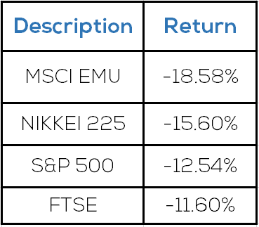
Above, the portfolio returns for the defined time periods are displayed. If the current bull market breaks with an increase in volatility which sees the level float to around 20, the sample portfolio is expected to lose 2.76%. If a more pronounced spike in volatility is seen and the VIX reaches the 40s a much larger loss can be expected, to the tune of 11.81%. The portfolio’s 11.81% loss during Q3 2011 is largely a result of equities falling across the board:

For a sanity check, we can use another of StatPro Revolutions risk tools, Alpha’s Market Stress. This steps the current portfolio through historical periods using a unique market model approach. Correlated stresses can be created to shock VIX up 100% to 20 and up 300% to 40. A correlated stress means the percentage increase in one market model parameter (VIX) is fixed, and the tool then automatically calculates the correlated shift in the other market model constituents. Using this approach, you can see the results below are similar for the first hypothetical, VIX to 20: a total loss of 2.22% made up primarily from equities but dampened by Fixed Income and FX trading gains.

The market stress tool may, however, underestimate the losses when the VIX level spikes to 40, for hypothetical 2 we see a loss of 7.78%. The discrepancy looks to be more conservative in the fact that we do not capture compounding losses which are a result of VIX’s sustained highs of 40.

_{Fig. 4: Market Stress pane within StatPro Alpha Module}

Conclusion

Volatility is a fact of investing, but at the same time it isn’t the only factor in determining a downturn. Scenarios and market stresses can be used to show possible outcomes for market volatility profiles. The historical scenarios are great for re-living specific market occurrences, but for the VIX to 40 example, the sample portfolio was being tested against one of the biggest sovereign debt crisis in recent history. The historical context of the scenario itself becomes an important factor as well.  With market stresses you are given more flexibility, for example if it was presumed that VIX to 40 would result in a less severe drop in the US Equity factor model parameter, it can be adjusted – essentially modifying the correlation of VIX to S&P 500.

Timing the end of the bull market and return of volatility is a question we may not be able to answer, but using StatPro’s risk management tools we are able to understand the magnitude of such events.

* Correct as of 11^th January 2018

{{cta(‘f543e487-b4d2-495c-a07a-cfa4a233f17e’)}}